## Import Libraries

import numpy as np
import pandas as pd
import altair as alt
from sklearn.datasets import load_breast_cancer
from sklearn.model_selection import train_test_split, GridSearchCV
from sklearn.preprocessing import StandardScaler
from sklearn.svm import SVC
from sklearn.metrics import accuracy_score, classification_report, confusion_matrix
from sklearn.naive_bayes import GaussianNB
import seaborn as sns
import matplotlib.pyplot as plt

Breast Cancer Detection (Tumor Classification with Support Vector Machines)
Purpose
The purpose of the created model is to detect accurately what type of tumor is found in the breast with the given features. The model will predict if the tumor is Malignant (cancerous).
## read in the data
cancer = pd.read_csv('https://raw.githubusercontent.com/davidorizu/files/main/breast_cancer.csv')
View the data
cancer.head()| id | diagnosis | radius_mean | texture_mean | perimeter_mean | area_mean | smoothness_mean | compactness_mean | concavity_mean | concave points_mean | ... | texture_worst | perimeter_worst | area_worst | smoothness_worst | compactness_worst | concavity_worst | concave points_worst | symmetry_worst | fractal_dimension_worst | Unnamed: 32 | |
|---|---|---|---|---|---|---|---|---|---|---|---|---|---|---|---|---|---|---|---|---|---|
| 0 | 842302 | True | 17.99 | 10.38 | 122.80 | 1001.0 | 0.11840 | 0.27760 | 0.3001 | 0.14710 | ... | 17.33 | 184.60 | 2019.0 | 0.1622 | 0.6656 | 0.7119 | 0.2654 | 0.4601 | 0.11890 | NaN |
| 1 | 842517 | True | 20.57 | 17.77 | 132.90 | 1326.0 | 0.08474 | 0.07864 | 0.0869 | 0.07017 | ... | 23.41 | 158.80 | 1956.0 | 0.1238 | 0.1866 | 0.2416 | 0.1860 | 0.2750 | 0.08902 | NaN |
| 2 | 84300903 | True | 19.69 | 21.25 | 130.00 | 1203.0 | 0.10960 | 0.15990 | 0.1974 | 0.12790 | ... | 25.53 | 152.50 | 1709.0 | 0.1444 | 0.4245 | 0.4504 | 0.2430 | 0.3613 | 0.08758 | NaN |
| 3 | 84348301 | True | 11.42 | 20.38 | 77.58 | 386.1 | 0.14250 | 0.28390 | 0.2414 | 0.10520 | ... | 26.50 | 98.87 | 567.7 | 0.2098 | 0.8663 | 0.6869 | 0.2575 | 0.6638 | 0.17300 | NaN |
| 4 | 84358402 | True | 20.29 | 14.34 | 135.10 | 1297.0 | 0.10030 | 0.13280 | 0.1980 | 0.10430 | ... | 16.67 | 152.20 | 1575.0 | 0.1374 | 0.2050 | 0.4000 | 0.1625 | 0.2364 | 0.07678 | NaN |
5 rows × 33 columns
cancer.columnsIndex(['id', 'diagnosis', 'radius_mean', 'texture_mean', 'perimeter_mean',
'area_mean', 'smoothness_mean', 'compactness_mean', 'concavity_mean',
'concave points_mean', 'symmetry_mean', 'fractal_dimension_mean',
'radius_se', 'texture_se', 'perimeter_se', 'area_se', 'smoothness_se',
'compactness_se', 'concavity_se', 'concave points_se', 'symmetry_se',
'fractal_dimension_se', 'radius_worst', 'texture_worst',
'perimeter_worst', 'area_worst', 'smoothness_worst',
'compactness_worst', 'concavity_worst', 'concave points_worst',
'symmetry_worst', 'fractal_dimension_worst', 'Unnamed: 32'],
dtype='object')## set target variable
cancer['diagnosis'] = cancer.diagnosis == "M"## inspect target variable
cancer["diagnosis"].unique()array([ True, False])## inspect data
cancer.info()<class 'pandas.core.frame.DataFrame'>
RangeIndex: 569 entries, 0 to 568
Data columns (total 33 columns):
# Column Non-Null Count Dtype
--- ------ -------------- -----
0 id 569 non-null int64
1 diagnosis 569 non-null bool
2 radius_mean 569 non-null float64
3 texture_mean 569 non-null float64
4 perimeter_mean 569 non-null float64
5 area_mean 569 non-null float64
6 smoothness_mean 569 non-null float64
7 compactness_mean 569 non-null float64
8 concavity_mean 569 non-null float64
9 concave points_mean 569 non-null float64
10 symmetry_mean 569 non-null float64
11 fractal_dimension_mean 569 non-null float64
12 radius_se 569 non-null float64
13 texture_se 569 non-null float64
14 perimeter_se 569 non-null float64
15 area_se 569 non-null float64
16 smoothness_se 569 non-null float64
17 compactness_se 569 non-null float64
18 concavity_se 569 non-null float64
19 concave points_se 569 non-null float64
20 symmetry_se 569 non-null float64
21 fractal_dimension_se 569 non-null float64
22 radius_worst 569 non-null float64
23 texture_worst 569 non-null float64
24 perimeter_worst 569 non-null float64
25 area_worst 569 non-null float64
26 smoothness_worst 569 non-null float64
27 compactness_worst 569 non-null float64
28 concavity_worst 569 non-null float64
29 concave points_worst 569 non-null float64
30 symmetry_worst 569 non-null float64
31 fractal_dimension_worst 569 non-null float64
32 Unnamed: 32 0 non-null float64
dtypes: bool(1), float64(31), int64(1)
memory usage: 142.9 KBMaking a heat map to view the relationship between variables.
## use seaborn library to make a heatmap
plt.figure(figsize=(9,8))
sns.heatmap(cancer.corr(), cmap="coolwarm", annot= False)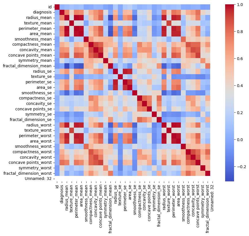
## make new dataset
cancer2=cancer

# make the features and target
features = ['radius_mean', 'texture_mean', 'perimeter_mean',
       'area_mean', 'compactness_mean', 'concavity_mean',
       'concave points_mean', 'symmetry_mean', 'fractal_dimension_mean',
       'radius_se', 'texture_se', 'perimeter_se', 'area_se', 'smoothness_se',
       'compactness_se', 'concavity_se', 'concave points_se', 'symmetry_se',
       'fractal_dimension_se', 'radius_worst', 'texture_worst',
       'perimeter_worst', 'area_worst', 'smoothness_worst',
       'compactness_worst', 'concavity_worst', 'concave points_worst',
       'symmetry_worst']

X = []
#X = pd.get_dummies(cancer2[cat])

X = cancer2[features]
y = cancer2['diagnosis']
Model Creation
# make x and y train and test
X_train, X_test, y_train, y_test = train_test_split(X, y, test_size=0.4, random_state=42)

# Standardize the feature values (mean=0, std=1)
scaler = StandardScaler()
X_train = scaler.fit_transform(X_train)
X_test = scaler.transform(X_test)
# Initialize the SVM model with an RBF kernel
svm_model = SVC(kernel='linear', random_state=42,C=0.1, gamma=1)
# Train the model
svm_model.fit(X_train, y_train)SVC(C=0.1, gamma=1, kernel='linear', random_state=42)In a Jupyter environment, please rerun this cell to show the HTML representation or trust the notebook.
On GitHub, the HTML representation is unable to render, please try loading this page with nbviewer.org.
SVC(C=0.1, gamma=1, kernel='linear', random_state=42)
Model Results
# Predict the test data
y_pred = svm_model.predict(X_test)

# Print evaluation metrics
print("Accuracy:", accuracy_score(y_test, y_pred))
print("Classification Report:\n", classification_report(y_test, y_pred, target_names=['malignant', 'benign']))
print("Confusion Matrix:\n", confusion_matrix(y_test, y_pred))
Accuracy: 0.9824561403508771
Classification Report:
precision recall f1-score support
malignant 0.99 0.99 0.99 148
benign 0.97 0.97 0.97 80
accuracy 0.98 228
macro avg 0.98 0.98 0.98 228
weighted avg 0.98 0.98 0.98 228
Confusion Matrix:
[[146 2]
[ 2 78]]## Visually showing the confusion matrix
import matplotlib.pyplot as plt
import itertools
cm = confusion_matrix(y_test, y_pred)
labels = ['malignant', 'benign'] # Your class labels
# Plot confusion matrix
plt.figure(figsize=(8, 6))
plt.imshow(cm, interpolation='nearest', cmap=plt.cm.Blues)
plt.title('Confusion Matrix')
plt.colorbar()
tick_marks = np.arange(len(labels))
plt.xticks(tick_marks, labels)
plt.yticks(tick_marks, labels)
thresh = cm.max() / 2.
for i, j in itertools.product(range(cm.shape[0]), range(cm.shape[1])):
plt.text(j, i, format(cm[i, j], 'd'),
horizontalalignment="center",
color="white" if cm[i, j] > thresh else "black")
plt.ylabel('True label')
plt.xlabel('Predicted label')
plt.tight_layout()
plt.show()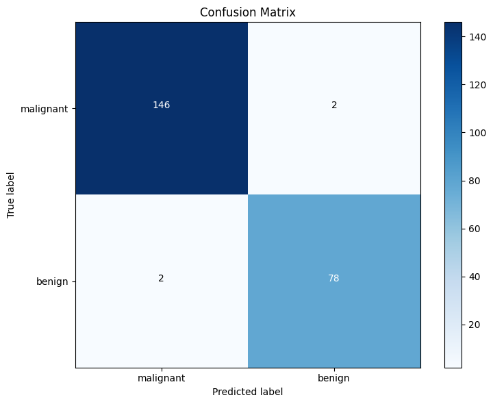
# Grid search
svm = SVC()
param_grid = {
    'C': [0.1, 1, 10, 100],
    'gamma': [1, 0.1, 0.01, 0.001],
    'kernel': ['linear', 'rbf', 'poly', 'sigmoid']
}

# Perform GridSearchCV to find the best hyperparameters
grid_search = GridSearchCV(svm, param_grid, cv=3, n_jobs=-1, verbose=2)
grid_search.fit(X_train, y_train)

# Get the best model from GridSearchCV
best_model = grid_search.best_estimator_
best_model
Fitting 3 folds for each of 64 candidates, totalling 192 fitsSVC(C=0.1, gamma=1, kernel='linear')In a Jupyter environment, please rerun this cell to show the HTML representation or trust the notebook.
On GitHub, the HTML representation is unable to render, please try loading this page with nbviewer.org.
SVC(C=0.1, gamma=1, kernel='linear')
import matplotlib.pyplot as plt

# Get the feature importance
feature_importance = abs(svm_model.coef_[0])

# Create a DataFrame for the feature importance
feature_importance_df = pd.DataFrame({
    'Feature': features,
    'Importance': feature_importance
})

# Sort the DataFrame by importance
feature_importance_df = feature_importance_df.sort_values(by='Importance', ascending=False)

# Plot the feature importance
plt.figure(figsize=(12, 8))
plt.barh(feature_importance_df['Feature'], feature_importance_df['Importance'], color='skyblue')
plt.xlabel('Feature Importance (absolute coefficient)')
plt.ylabel('Feature')
plt.title('Feature Importance for Breast Cancer Diagnosis using SVM')
plt.gca().invert_yaxis()
plt.show()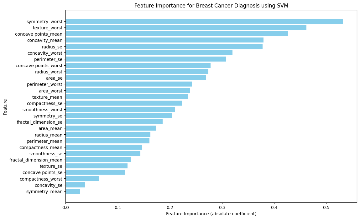
How other models compare:
# Initialize the Naive Bayes model
nb_model = GaussianNB()

# Train the model
nb_model.fit(X_train, y_train)

# Predict the test data
y_pred = nb_model.predict(X_test)

# Print evaluation metrics
print("Accuracy:", accuracy_score(y_test, y_pred))
print("Classification Report:\n", classification_report(y_test, y_pred, target_names=['malignant', 'benign']))
Accuracy: 0.9517543859649122
Classification Report:
precision recall f1-score support
malignant 0.95 0.97 0.96 148
benign 0.95 0.91 0.93 80
accuracy 0.95 228
macro avg 0.95 0.94 0.95 228
weighted avg 0.95 0.95 0.95 228
Confusion Matrix:
[[144 4]
[ 7 73]]# create tree
from sklearn.tree import DecisionTreeClassifier
clf = DecisionTreeClassifier()
# train tree
clf.fit(X_train, y_train)
y_pred = clf.predict(X_test)
print("Accuracy:", accuracy_score(y_test, y_pred))
print("Classification Report:\n", classification_report(y_test, y_pred, target_names=['malignant', 'benign']))Accuracy: 0.9298245614035088
Classification Report:
precision recall f1-score support
malignant 0.96 0.93 0.94 148
benign 0.87 0.94 0.90 80
accuracy 0.93 228
macro avg 0.92 0.93 0.92 228
weighted avg 0.93 0.93 0.93 228
Confusion Matrix:
[[137 11]
[ 5 75]]from sklearn.neighbors import KNeighborsClassifier
# Initialize the KNeighborsClassifier model
kn_model = KNeighborsClassifier()
# Train the model
kn_model.fit(X_train, y_train)
# Predict the test data
y_pred = kn_model.predict(X_test)
# Print evaluation metrics
print("Accuracy:", accuracy_score(y_test, y_pred))
print("Classification Report:\n", classification_report(y_test, y_pred, target_names=['malignant', 'benign']))Accuracy: 0.9605263157894737
Classification Report:
precision recall f1-score support
malignant 0.98 0.96 0.97 148
benign 0.93 0.96 0.94 80
accuracy 0.96 228
macro avg 0.95 0.96 0.96 228
weighted avg 0.96 0.96 0.96 228
Confusion Matrix:
[[142 6]
[ 3 77]]data = {
'model': ['Support Vector Machine(SVM)', 'KNeighborsClassifier', 'Naive Bayes', 'DecisionTreeClassifier'],
'accuracy': [0.982456, 0.9605, 0.95175, 0.92982]
}
data_accuracy = pd.DataFrame(data)
data = {
'model': ['Support Vector Machine(SVM)', 'Naive Bayes', 'KNeighborsClassifier', 'DecisionTreeClassifier'],
'recall': [0.99, 0.97, 0.96, 0.93]
}
data_recall = pd.DataFrame(data)alt.Chart(data_accuracy).mark_bar().encode(
alt.X('accuracy', title="Accuracy", scale = alt.Scale(domain=(0.5,1))),
alt.Y('model', title='', sort=alt.EncodingSortField(field="accuracy", order="descending")),
color='model'
).properties(
title='Accuracy Score for each potential model'
)alt.Chart(data_recall).mark_bar().encode(
alt.X('recall', title="Recall Score", scale = alt.Scale(domain=(0.5,1))),
alt.Y('model', title='', sort=alt.EncodingSortField(field="recall", order="descending")),
color='model'
).properties(
title='Recall Score for each potential model'
)alt.Chart(cancer2).mark_boxplot().encode(
alt.Y('diagnosis', title="Malignant"),
alt.X('symmetry_worst', title='symmetry_worst'),
alt.Color('diagnosis:N',title='Malignant')
).properties(
title='Boxplot of symmetry_worst for malignant and benign tumors'
)